1. Introduction

Linear regression is interpretable and well-studied. I present to you a rough anthology of linear regression.¹ By this, I mean several different approaches to linear regression. We’ll start off with minimizing MSE and end up with a Bayesian approach with hopefully a (semi-)rigorous approach throughout. Ideally, everything should feel motivated.

There are several computational tricks / alternative derivations which are shorter and easier. I’ll go through some of them at the end of the article but it’s probably valuable to do it the painful way at least once.

2. Problem Set up

We begin with a dataset $\mathcal{D} = {(x_i, y_i)}_{i= 1}^n$. Let $y \in \mathbb{R}, x \in \mathbb{R}^d$. We want to find a linear relationship between features $x_i$ and noisy target values $y_i$, i.e.:

\[y_i = f(x_i) + \epsilon_x\]

If we believe the underlying relationship between $y$ and $x$ is in fact linear, we set

\[f(x_i) = w^T x_i\]

where $w$ represents the weights or scaling coefficients.

We can collect the target values $y_1, \dots, y_n$ into a vector $y$ and the feature vectors $x_1, \dots, x_N$ into a design matrix $X$ where the row $X_i = x_i$. This ensures each $y_i = x_i^T w$.

\[y = X w + \epsilon_x\]

Note that this represents $y$ as a column vector.

3. Minimize MSE

The first perspective on linear regression is just minimizing the error between the targets $y$ and the predictions $Xw$. We’ll derive this with matrix calculus².The residual (error between $Xw$ and $y$) is defined as:

\[e = y - Xw\]

We want to find the $\hat{w}$ that minimizes the mean-squared error:

\[\hat{w} = \argmin_{w} \ e^T e = \argmin_{w} \ (y - Xw)^T (y - Xw)\]

For optimization problems like this, we can just take the first derivative w.r.t $w$ and set to $0$.

\[0 = \frac{\partial e^T e}{\partial w} = \frac{\partial}{\partial w} (y - Xw)^T (y - Xw)\] \[= \frac{\partial}{\partial w} (y^T y + w^T X^T X w - 2 w^T X^T y)\]

There are two ways to treat matrix derivatives. Numerator layout (treating the gradient as row vector) and denominator layout (treating the gradient as a column vector). This actually caused me great grief when I was learning this on my own but I’ve kinda gotten over it. So both views are presented here.

Here are the rules we will use (treating the gradient as a row vector). To treat the gradient as a column vector, take the transpose.

\[\frac{\partial}{\partial x} x^T a = \frac{\partial}{\partial x} a^T x = a^T\] \[\frac{\partial}{\partial x} x^T A x = x^T (A + A^T)\]

To verify these rules for yourself, you can just convert these matrix-vector products into sums.

3.1 Gradient is a Row Vector

The first term ($y^T y$) is not dependent on $w$ so it goes to zero. The second term becomes $2 w^T X^T X$. The third term becomes $2 y^T X$. So we have:

\[0 = 2 w^T X^T X - 2 y^T X\] \[y^T X = w^T X^T X\] \[w^T = y^T X (X^T X)^{-1}\] \[w = (X^T X)^{-1} X^T y\]

If a symmetric matrix is non-singular, it’s inverse is also symmetric.

3.2 Gradient is a Column Vector

The second term becomes $2 X^T X w$ and the third becomes $2 X^T y$.

\[0 = 2 X^T X w - 2 X^T y\]

Skipping ahead…

\[w = (X^T X)^{-1} X^T y\]

Okay, this was all fairly simple. We can also read this as $w = \frac{\text{Cov}(X, y)}{\text{Var}(X)}$ to view this from another, probabilistic angle.

I hope everything seems relatively well-motivated thus far. However, there are certain assumptions that have already been made as well as other issues that have been glossed over.

Prominently, we defined the loss function to be the mean-squared error $\text{MSE}(y, Xw)$. This is equivalent to minimizing the $L_2$ norm of the residuals. But why use mean-squared error? Why not mean absolute error (MAE) or mean-cubic error?

There are many reasons why MSE is a empirically nice loss function to use. It’s differentiable unlike MAE and doesn’t place as much weight on outliers as mean errors of higher order terms does. $L_2$ is also a Hilbert space while $L_p$ for $p \geq 1, p \neq 2$ is not (whatever that means). But we still chose MSE. These are justifications, not derivations from first principles.

I find that everything fits better in my head when we don’t choose an arbitrary loss function but are forced into that choice from the assumptions we make. My professor once said (paraphrasing) being Bayesian is all about being up-front and honest with our beliefs. We want to honestly represent our assumptions here. A good first step towards that is to do linear regression probabilistically (we’ll get to the Bayesian bits eventually).

4. Maximum Likelihood Estimation

Let’s begin by placing a distribution over the noise. Say, for example, we choose $\epsilon_x \sim \mathcal{N}(0, \sigma^2)$. So we have:

\[\epsilon_x \sim \mathcal{N}(0, \sigma^2)\] \[y_i \sim \mathcal{N}(w^T x_i, \sigma^2)\]

The likelihood function is:

\[\mathcal{L}(w \mid \mathcal{D}) = p(\mathcal{D} \mid w)\]

We want to maximize the likelihood of observing the data (what does this mean?). Our data points $y_i$ are i.i.d. since they’re all drawn from $\mathcal{N}(w^T x_i, \sigma^2)$ (identical) and are conditionally independent on the mean and variance. So we have:

\[p(\mathcal{D} \mid w) = p(y_1, \dots, y_N \mid w, x_1, \dots, x_n, \sigma^2)\] \[= \prod_{i = 1}^n \mathcal{N}(y_i ; w^T x_i, \sigma^2)\] \[= \prod_{i = 1}^n \frac{1}{\sqrt{2 \pi \sigma^2}} \exp \left \{ - \frac{1}{2 \sigma^2} (y_i - w^T x_i)^2 \right \}\]

The product of exponentials becomes a sum within the exponential. So we have:

\[= \frac{1}{(2 \pi \sigma^2)^\frac{n}{2}} \exp \left \{ - \frac{1}{2 \sigma^2} \sum_{i = 1}^n (y_i - w^T x_i)^2 \right \}\]

We can re-write these as inner products and save ourselves a lot of mental load. A physics PhD student I was working with actually pointed this out to me and I never looked back (thank you!)

\[= \frac{1}{(2 \pi \sigma^2)^\frac{n}{2}} \exp \left \{ - \frac{1}{2 \sigma^2} (y - Xw)^T (y - Xw) \right \}\]

Now, we want to maximize this likelihood with respect to $w$. Since the logarithm is a monotonic transformation, the log-likelihood and the likelihood have the same extrema. So, we have:

\[w_{\text{MLE}} = \argmax_w \ p(\mathcal{D} \mid w) = \argmax_w \ \log p(\mathcal{D} \mid w)\]

So we have:

\[\log p(\mathcal{D} \mid w) = - \frac{1}{2 \sigma^2} (y^Ty + w^T X^T X w - 2 y^T X w) - \frac{n}{2} \log(2 \pi \sigma^2)\] \[0 = \frac{\partial}{\partial w} \log p(D \mid w) = - \frac{1}{2 \sigma^2} \frac{\partial}{\partial w} (y^T y + w^T X^T X w - 2 y^T X w)\]

For convenience’s sake, I’ll treat the gradient as a column vector although I generally prefer the other way.

So we have:

\[0 = 2 X^T X w - 2 X^T y\] \[X^T y = X^T X w\] \[w_{\text{MLE}} = (X^T X)^{-1} X^T y\]

This is no different from what we’ve already seen. But we can also derive a maximum likelihood estimate for the noise variance.

\[0 = \frac{\partial}{\partial \sigma^2} \log p(\mathcal{D} \mid w) = \frac{\partial}{\partial \sigma^2} \left [ - \frac{1}{2 \sigma^2} (y^Ty + w^T X^T X w - 2 y^T X w) - \frac{n}{2} \log(2 \pi \sigma^2) \right ]\] \[0 = - \frac{2 n \pi}{4 \pi \sigma^2} + \frac{1}{2 \sigma^4} (y - Xw)^T (y - Xw)\] \[\frac{n}{\sigma^2} = \frac{1}{\sigma^4} (y - Xw)^T (y - Xw)\] \[\sigma^2_{\text{MLE}} = \frac{1}{n} (y - Xw)^T (y - Xw)\]

This is a little better - its nice to be able to estimate the variance of the noise as well.

Math is nice but we need to check whether or not this formula actually works. We implement these basic formulas to generate the following image.

import torch
import matplotlib.pyplot as plt

torch.manual_seed(42)

x = 30.0 * torch.rand(100)
y = 3.0 * x + 40.0 + torch.randn(100) * torch.sqrt(torch.tensor(5.0))

X = torch.stack([torch.ones(100), x], dim=1)

w_MLE = torch.linalg.inv(X.T @ X) @ X.T @ y
y_pred = X @ w_MLE

sigma_2_mle = ((y - y_pred).T @ (y - y_pred)) / (100 - 2)
slope_str = f"Estimated Slope, Intercept, Noise Variance: {w_MLE[1]:.4f}, {w_MLE[0]:.4f}, {sigma_2_mle:.4f}, True Noise Variance: {5.0:.4f}"
# Estimated Slope: 2.9656, Intercept: 40.5160, Noise Variance: 3.3836, True Noise Variance: 5.0000

plt.title(slope_str, fontsize=10, color="black")
plt.plot(x, y, "o", label="Noisy Targets", color="blue")
plt.plot(x, y_pred, "-*",label="Predictions", color="red")
plt.legend()
plt.show()

MLE Linear Regression

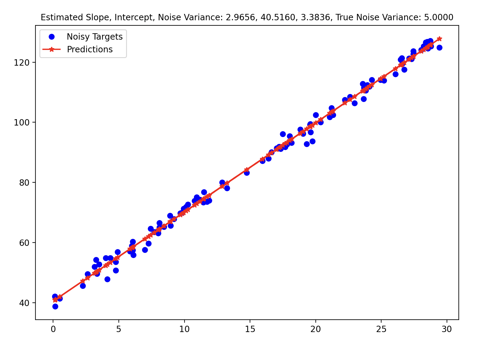
However, the MLE of the variance is a biased estimator. Bessel’s correction divides $(y - Xw)^T (y - Xw)$ by $(n - p)$ where $p$ is the number of degrees of freedom to get a unbiased estimator (in the above case, $p = 2$ - slope, intercept). The following GIF shows how different estimators of the variance change w.r.t. different variances. To be honest, I initially found that the MLE / Bessel estimators were initially overestimating variance but figured out this was because of the random seed. Over different random seeds, the MLE estimator tended to generally underestimate the true noise variance.

Variance Estimator GIF

The code for that can be found here.

4.1 Issues with MLE

There are several issues with maximum likelihood estimation. But the most glaring one, to me at least, is that it fundamentally answers the wrong question. Do we really care about the probability of the data given some parameter setting? I think the more natural question is the probability of some parameter setting given the data.

5. MAP

One way to do this is with MAP or Maximum a Posteriori estimation.

Bayes Rule states:

\[p(w \mid \mathcal{D}) = \frac{p(\mathcal{D} \mid w) p(w)}{p(\mathcal{D})}\]

The left-hand side is called the posterior distribution. It’s proportional to the likelihood multiplied with the prior distribution. The prior represents our beliefs about the data before we have observed the data - the posterior represents our updated beliefs after having observed the data (likelihood).

So we need to place a prior distribution on $w$. So we can specify:

\[w \sim \mathcal{N}(0, \alpha^2 I)\] \[\epsilon_x \sim \mathcal{N}(0, \sigma^2)\]

So the joint distribution can be written as a multivariate Gaussian.

\[y \mid w, X, \sigma^2 \sim \mathcal{N}(Xw, \sigma^2 I)\]

The MAP estimate $w_{\text{MAP}}$ is the parameter setting which maximizes the probability of the parameter given the data. So we want:

\[w_{\text{MAP}} = \argmax_{w} \ p(w \mid \mathcal{D})\]

Again, we can take the logarithm, so we have:

\[w_{\text{MAP}} = \argmax_{w} \ \log p(w \mid \mathcal{D})\] \[= \argmax_{w} \ \log p(\mathcal{D} \mid w) + \log p(w) - \log(\mathcal{D})\]

The denominator of Bayes rule is called the marginal likelihood or the partition function or the evidence. Since it doesn’t depend on $w$, we can just ignore it in finding $w_{\text{MAP}}$. So we have:

\[0 = \frac{\partial}{\partial w} \log p(\mathcal{D} \mid w) + \log p(w)\]

Taking the logarithm of normal distributions,

\[= \frac{\partial}{\partial w} \left [ - \frac{1}{2 \sigma^2} (y - Xw)^T (y - Xw) - \frac{n}{2} \log (2 \pi \sigma^2) - \frac{1}{2 \alpha^2} w^T w - \frac{d}{2} \log (2 \pi \alpha^2) \right ]\]

We’ve performed bits and pieces of this derivative above. So we get

\[0 = \frac{X^T y}{\sigma^2} - \frac{w}{\alpha^2} - \frac{X^T X w}{\sigma^2}\] \[0 = X^T y - \frac{\sigma^2 w}{\alpha^2} - X^T X w\]

Define $\lambda = \frac{\sigma^2}{\alpha^2}$. Then, we have:

\[0 = X^T y - \lambda w - X^T X w\] \[(X^T X + \lambda I)w = X^T y\] \[w_{\text{MAP}} = (X^T X + \lambda I)^{-1} X^T y\]

We can reach this formula by finding:

\[w_{\text{MAP}} = \argmin_{w} (y - Xw)^T (y - Xw) + \lambda w^T w\]

In other words, we can recover $L_2$ regularization by assuming Gaussian noise and a Gaussian prior. I like this probabilistic approach much better because it all feels very motivated from our assumptions.

We can also derive MAP solutions for the noise and weight variances. The MAP solution for the noise variance is the same as the MLE solution because it’s not affected by the prior.

\[0 = \frac{\partial}{\partial \alpha^2} \left [ - \frac{1}{2 \alpha^2} w^T w - \frac{d}{2} \log (2 \pi \alpha^2) \right ]\] \[= \frac{1}{2 \alpha^4} w^T w - \frac{d}{2 \alpha^2}\] \[\alpha^2_{\text{MAP}} = \frac{1}{d} w_{\text{MAP}}^T w_{\text{MAP}}\]

Let’s gut-check. If we send the prior variance of the weight to $0$, i.e. $\alpha^2 \to 0$, then the regularization coefficient $\lambda$ grows very large so the weights move towards $0$. Similarly, if we send the noise variance $\sigma^2 \to \infty$, we will see a similar result.

6. Bayesian Linear Regression

6.1 Marginal Likelihood

I want to talk briefly about the marginal likelihood (evidence, partition function, normalizing constant) which is the denominator in Bayes rule. By the sum and product rules of probability, we have:

\[p(\mathcal{D}) = \int p(\mathcal{D} \mid w) \ p(w) \ dw\]

By marginalizing out $w$ (hence the name marginal likelihood), we get a term which tells us the likelihood of the data, conditioned on hyperparameters. This also lets us directly perform hyperparameter optimization. Contrast optimizing this quantity with other hyperparameter optimization techniques like grid search which is exponential in the number of hyperparameter-combinations or random search which is … random.

Of course, the downside of this method (marginal likelihood optimization or Type 2 MLE) is that it involves an integral which is often intractable.

We’ll use the same prior and noise distribution as before and compute the marginal likelihood. Buckle up.³

\[p(\mathcal{D}) = \int \mathcal{N}(y ; Xw, \sigma^2 I) \ \mathcal{N}(w ; 0, \alpha^2 I) \ dw\] \[= c \int \exp \left \{ - \frac{1}{2} \left [ \frac{(y - Xw)^T (y - Xw)}{\sigma^2} + \frac{w^T w}{\alpha^2} \right ] \right \} \ dw\] \[= c \int \exp \left \{ - \frac{1}{2} \left [ \frac{y^T y + w^T X^T X w - 2 w^T X^T y}{\sigma^2} + \frac{w^T w}{\alpha^2} \right ] \right \} dw\]

The strategy here is to transform the exponential inside the integrand into an unnormalized probability distribution, or the posterior, $p(w \mid \mathcal{D}) \propto p(\mathcal{D} \mid w) p(w)$. Moving the $y^T y$ term out of the integral (since it doesn’t depend on $ws), we get:

\[= c' \int \exp \left \{ - \frac{1}{2} \left [ \frac{w^T X^T X w - 2 w^T X^T y}{\sigma^2} + \frac{w^T w}{\alpha^2} \right ] \right \} dw\] \[= c' \int \exp \left \{ - \frac{1}{2} \left [ w^T \left ( \frac{X^T X}{\sigma^2} + \frac{I}{\alpha^2} \right ) w - \frac{2 w^T X^T y}{\sigma^2} \right ] \right \} dw\]

We can infer the precision matrix $\Lambda = \frac{X^T X}{\sigma^2} + \frac{I}{\alpha^2}$. We want the integrand to be (ignoring the exponential), of the form $(w - \mu)^T \Lambda (w - \mu)$. We have:

\[(w - \mu)^T \Lambda (w - \mu) = w^T \Lambda w + \mu^T \Lambda \mu - 2 w^T \Lambda \mu\]

By inspection, we know that $2 w^T \Lambda \mu = \frac{2 w^T X^T y}{\sigma^2}$. So we have $\Lambda \mu = \frac{X^T y}{\sigma^2}, \mu = \Lambda^{-1} \frac{X^T y}{\sigma^2}$.

So we have:

\[w^T \Lambda w - 2 w^T \Lambda \mu = (w - \mu)^T \Lambda (w - \mu) - \mu^T \Lambda \mu\]

So we have:

\[p(\mathcal{D}) = c' \int \exp \left \{ - \frac{1}{2} \left [ (w - \mu)^T \Lambda (w - \mu) - \mu^T \Lambda \mu \right ] \right \} \ dw\]

Finally, we can take out the term $\mu^T \Lambda \mu$ to get:

\[p(\mathcal{D}) = c'' \int \exp \left \{ - \frac{1}{2} (w - \mu)^T \Lambda (w - \mu) \right \} \ dw\]

There’s a nice integral trick to know here. If we have a probability distribution $f(x) = \frac{\hat{f}(x)}{Z}$ where $Z$ is the normalizing constant, it follows that the integral of the unnormalized probability distribution is $\int \hat{f} (x) \ dx = \frac{1}{Z}$.

The integrand corresponds to an unnormalized normal distribution $\mathcal{UN}(w; \mu, \Lambda^{-1})$ (my own notation :P). So we have:

\[\int \exp \left \{ - \frac{1}{2} (w - \mu)^T \Lambda (w - \mu) \right \} \ dw = (2 \pi )^{\frac{d}{2}} \det(\Lambda^{-1})^{\frac{1}{2}}\] \[= \frac{(2 \pi )^{\frac{d}{2}}}{\det(\Lambda)^{\frac{1}{2}}}\]

Finally, we’ve reached a closed form solution.

\[p(\mathcal{D}) = c'' \frac{(2 \pi )^{\frac{d}{2}}}{\det(\Lambda)^{\frac{1}{2}}}\] \[= \frac{\exp \left \{ - \frac{1}{2} \left [ \frac{y^T y}{\sigma^2} + \mu^T \Lambda \mu \right ] \right \}}{(2 \pi \sigma^2)^{\frac{n}{2}} (2 \pi \alpha^2)^{\frac{d}{2}}} \frac{(2 \pi )^{\frac{d}{2}}}{\det(\Lambda)^{\frac{1}{2}}}\]

However, we can again, re-write this slightly. First of all, observe that:

\[\mu^T \Lambda \mu = \frac{y^T X}{\sigma^2} \Lambda^{-1} \Lambda \Lambda^{-1} \frac{X^T y}{\sigma^2}\] \[= \frac{y^T X \Lambda^{-1} X^T y}{\sigma^4}\]

So let’s re-write the term in this exponential as:

\[p(\mathcal{D}) = \frac{\exp \left \{ - \frac{1}{2} y^T \left [ \frac{I}{\sigma^2} + \frac{X \Lambda^{-1} X^T}{\sigma^4} \right ] y \right \}}{(2 \pi \sigma^2)^{\frac{n}{2}} (2 \pi \alpha^2)^{\frac{d}{2}}} \frac{(2 \pi )^{\frac{d}{2}}}{\det(\Lambda)^{\frac{1}{2}}}\]

Define $\Lambda_0 = \frac{I}{\sigma^2} + \frac{X \Lambda^{-1} X^T}{\sigma^4}$. So we have

\[p(\mathcal{D}) = \frac{\exp \left \{ - \frac{1}{2} y^T \Lambda_0 y \right \}}{(2 \pi \sigma^2)^{\frac{n}{2}} (2 \pi \alpha^2)^{\frac{d}{2}}} \frac{(2 \pi )^{\frac{d}{2}}}{\det(\Lambda)^{\frac{1}{2}}}\]

We can honestly leave it here. But we won’t because we know there is a Gaussian distribution hiding somewhere in there. I’m gonna go ahead and take a shot in the dark that $p(\mathcal{D}) = \mathcal{N}(0, \Lambda_0^{-1})$. Let’s test that hypothesis.

I’ll introduce two lemmas which are generally quite useful in Bayesian statistics. The first one is the Woodbury Matrix Identity. It states:

\[(A + UCV)^{-1} = A^{-1} - A^{-1} U (C^{-1} + V A^{-1} U)^{-1} V A^{-1}\]

Define $C = \frac{\Lambda^{-1}}{\sigma^4}, U = -X, V = X^T, A = \frac{I}{\sigma^2}$. Then, we have:

\[\Lambda_0^{-1} = \sigma^2 I + \sigma^2 I X (\sigma^4 \Lambda - \sigma^2 X^T X)^{-1} X^T \sigma^2 I\]

Substitute in $\Lambda = \frac{X^T X}{\sigma^2} + \frac{I}{\alpha^2}$.

\[\Lambda_0^{-1} = \sigma^2 I + \sigma^4 X \left (\sigma^4 \left ( \frac{X^T X}{\sigma^2} + \frac{I}{\alpha^2} \right ) - \sigma^2 X^T X \right )^{-1} X^T\] \[\Lambda_0^{-1} = \sigma^2 I + \sigma^4 X \left ( \sigma^2 X^T X + \frac{\sigma^4}{\alpha^2} I - \sigma^2 X^T X \right )^{-1} X^T\] \[= \sigma^2 I + \sigma^4 X \left ( \frac{\sigma^4}{\alpha^2} I \right )^{-1} X^T\] \[= \sigma^2 I + \alpha^2 X X^T\]

When I derived this for the first time, I was actually surprised by how nice this matrix inverse is.⁴

Next, let’s compute the determinant of this. What I’m hoping for is that the determinant of the covariance matrix will absorb some of the straggling terms in the normalizing coefficient(s). Recall, we have:

\[p(\mathcal{D}) = \frac{\exp \left \{ - \frac{1}{2} y^T \Lambda_0^{-1} y \right \}}{(2 \pi \sigma^2)^{\frac{n}{2}} (2 \pi \alpha^2)^{\frac{d}{2}}} \frac{(2 \pi )^{\frac{d}{2}}}{\det(\Lambda)^{\frac{1}{2}}}\]

First, we can immediately cancel out $(2 \pi)^{\frac{d}{2}}$.

\[p(\mathcal{D}) = \frac{\exp \left \{ - \frac{1}{2} y^T \Lambda_0^{-1} y \right \}}{(2 \pi \sigma^2)^{\frac{n}{2}} (\alpha^2)^{\frac{d}{2}} \det(\Lambda)^{\frac{1}{2}}}\]

So now, we’ll use the determinant lemma to compute $\det(\Lambda_0^{-1})$. The determinant lemma states:

\[\det(A + UWV^T) = \det(W^{-1} + V^T A^{-1} U) \det(W) \det(A)\] \[\det(\sigma^2 I + X \alpha^2 I X^T) = \det(\frac{I}{\alpha^2} + X^T \frac{I}{\sigma^2} X) \det(\alpha^2 I) \det (\sigma^2 I)\]

Recall that $\Lambda = \frac{I}{\alpha^2} + \frac{X^T X}{\sigma^2}$. So we have:

\[\det(\Lambda_0^{-1}) = \det(\Lambda) (\alpha^2)^{d} (\sigma^2)^{n}\] \[\det(\Lambda_0^{-1})^{\frac{1}{2}} = \det(\Lambda)^{\frac{1}{2}} (\alpha^2)^{\frac{d}{2}} (\sigma^2)^{\frac{n}{2}}\]

So in conclusion, we have:

\[p(\mathcal{D}) = \frac{\exp \left \{ - \frac{1}{2} y^T \Lambda_0^{-1} y \right \}}{(2 \pi)^{\frac{n}{2}} \det(\Lambda_0^{-1})^{\frac{1}{2}}}\] \[\boxed{\mathcal{D} \sim \mathcal{N}(y; 0, \sigma^2 I + \alpha^2 X X^T)}\]

Phew. This evidence quantity is very hard to compute so we try and avoid it best we can. But with nice models like linear-Gaussian, we can do it.

Fun fact: the marginal likelihood is often written with a $Z$ because it stands for Zustandssumme or “sum over states” in German.

6.2 Posterior Distribution

Finally, let’s compute the normalized posterior distribution. Specifically, we want $p(w \mid \mathcal{D})$. Good news - we’ve already done this! The integrand of the marginal likelihood is our answer: we have,

\[p(w \mid \mathcal{D}) = \mathcal{N}(\mu, \Lambda^{-1})\] \[\Lambda = \frac{X^T X}{\sigma^2} + \frac{I}{\alpha^2}\] \[\mu = \Lambda^{-1} \frac{X^T y}{\sigma^2}\]

There are very simple ways to derive this from Gaussian identities.⁵ But since most of the work is already kind of done for us, let’s derive it the “hard” way.

\[p(w \mid \mathcal{D}) = \frac{p(\mathcal{D} \mid w) p(w)}{p(\mathcal{D})}\] \[= \frac{\mathcal{N}(y; Xw, \sigma^2 I) \mathcal{N}(w; 0, \alpha^2 I)}{\mathcal{N}(y; 0, \alpha^2 X X^T + \sigma^2 I)}\]

From the previous section, we can write the denominator:

\[D_e = \frac{(2 \pi \sigma^2)^{\frac{n}{2}} \det(\Lambda)^{\frac{1}{2}} (\alpha^2)^{\frac{D}{2}}}{\exp(- \frac{1}{2} [ \frac{y^T y}{\sigma^2} - \mu^T \Lambda \mu])}\]

and the numerator:

\[N_u = \frac{\exp \left \{ - \frac{1}{2 \sigma^2} (y - Xw)^T (y - Xw) - \frac{1}{2 \alpha^2} w^T w \right \}}{(2 \pi \sigma^2)^{\frac{n}{2}} (2 \pi \alpha^2)^{\frac{D}{2}}}\]

Now, most of the constants cancel out except for $(2 \pi)^{\frac{D}{2}}$ and $\det(\Lambda)^{\frac{1}{2}}$. Let $E(w)$ be the argument inside the exponential.

\[\frac{N_u}{D_e} = \frac{E(w)}{\sqrt{(2 \pi)^D \det(\Lambda^{-1})}}\]

Finally, let’s put an end to this long fight and compute $E(w)$. Just be careful about signs.

\[E(w) = - \frac{1}{2} \left [ \frac{(y - Xw)^T(y - Xw)}{\sigma^2} + \frac{w^T w}{\alpha^2} + \mu^T \Lambda \mu - \frac{y^T y}{\sigma^2} \right ]\] \[E(w) = - \frac{1}{2} \left [ \frac{y^T y + w^T X^T X w - 2 w^T X^T y}{\sigma^2} + \frac{w^T w}{\alpha^2} + \mu^T \Lambda \mu - \frac{y^T y}{\sigma^2} \right ]\]

Canceling out the $\frac{y^T y}{\sigma^2}$ terms,

\[= - \frac{1}{2} \left [ w^T \left (\frac{X^T X}{\sigma^2} + \frac{I}{\alpha^2} \right ) w - 2 \frac{w^T X^T y}{\sigma^2} + \mu^T \Lambda \mu \right ]\] \[= - \frac{1}{2} \left [ w^T \Lambda w - 2 w^T \Lambda \mu + \mu^T \Lambda \mu \right ]\]

In completing the square in the previous section, we found this to be equal to:

\[= - \frac{1}{2} \left [ (w - \mu)^T \Lambda (w - \mu) - \mu^T \Lambda \mu + \mu^T \Lambda \mu \right ]\] \[= - \frac{1}{2} \left [ (w - \mu)^T \Lambda (w - \mu) \right ]\]

So we have:

\[p(w \mid \mathcal{D}) = \frac{\exp(- \frac{1}{2} (w - \mu)^T \Lambda (w - \mu))}{\sqrt((2 \pi)^{D} \det(\Lambda^{-1}))}\] \[\boxed{w \mid \mathcal{D} \sim \mathcal{N}(\mu, \Lambda^{-1})}\]

So we have an estimate for $w$. But how do we actually make point predictions?

6.3 Predictive Distribution

The predictive distribution is pretty simple.

\[p(y_* \mid X_*, \alpha^2, \sigma^2, \mathcal{D}) = \int p(y_* \mid X_*, w, \sigma^2) p(w \mid \mathcal{D}, \alpha^2) dw\]

This is called the Bayesian Model Average. It is robust to overfitting and I like it very much. It weights our predictions for different output points $y_*$ by the posterior probability of the coefficient $w$.

7. Conclusion

This post is long with a lot of tedious math so if you got through it, I think you should feel proud. We went over linear regression with MSE, MAP, and the BMA which is quite a lot. I hope you learned something too! I would estimate that the knowledge in this post probably took around 9 months to accumulate? Obviously, this is not the best metric for how long it takes to learn these different perspectives because I wasn’t actively seeking out said perspectivesduring those 9 months. I learned the standard MSE perspective in my first machine learning class and then MAP and the BMA I learned in a Bayesian machine learning class. Very interesting stuff.

Just a note on marginal likelihood optimization (also called empirical bayes or Type 2 MLE). The marginal likelihood answers a subtly different question than what one might want. I believe it relates to the likelihood of the training data under a prior model rather than questions of which hyperparameters generalize best. Still, it’s often treated as a proxy to such.

8. Footnotes

All of these examples work with feature transformations on $X$, i.e. replacing $X$ with $\Phi$. Linear regression is super powerful… when it can be made non-linear! ↩
Linear algebra is your friend. Probably your best friend, actually. It allows a very easy and simple derivation of linear regression.

We know that $y$ is a vector and the solution $X w$ is the vector which is closest to $y$. In other words, $y$ is an orthogonal projection onto $\text{span}(X)$. This means the error vector $e = y - Xw$ is orthogonal to $X$. So we have:
\[X^T e = 0\] \[X^T (y - Xw) = 0\] \[X^T y - X^T X w = 0\] \[w = (X^T X)^{-1} X^T y\]
↩
Bayesian statistics math is notoriously tedious. There’s a much easier way to do this by treating it as a Gaussian Process. I’ll derive it quickly here. Suppose $w \sim \mathcal{N}(0, \alpha^2 I), \epsilon_x \sim \mathcal{N}(0, \sigma^2 I)$.
\[y = Xw + \epsilon_x\] \[E[y]= E[Xw] + E[\epsilon_x]\]
$E[\epsilon_x] = 0$ since it has mean $0$. For the same reason,
\[E[Xw] = X E[w] = 0\]
So $E[y] = 0$. Next, we’ll compute the covariance matrix.
\[E[y y^T] = E[(Xw + \epsilon_x)(Xw + \epsilon_x)^T]\]
Order matters here. These are all matrices so we cannot interchange the order of multiplication between $Xw$ and $w^T X^T$.
\[= E[Xw w^T X^T + \epsilon_x \epsilon_x^T + \epsilon_x w^T X^T + X w \epsilon_x^T ]\]
The other terms go to $0$. Since $\epsilon_x$ and $w$ are independent, $E[\epsilon_x w] = E[\epsilon] E[w]$ = 0.
\[= X E[ww^T] X^T + E[\epsilon_x \epsilon_x^T]\] \[= \sigma^2 I + \alpha^2 X X^T\]
Much easier… : ) ↩
Sometimes it’s a lot nicer to use the precision matrix (inverse of covariance matrix). I kind of want to make a post later about what the precision matrix actually means - it has something to do with partial correlations. Here, the precision matrix is quite ugly but the covariance matrix is really nice. ↩
Once we know the mean $\mu$ and precision matrix $\Lambda$, we can kind of just infer that $w \mid \mathcal{D} \sim \mathcal{N}(\mu, \Lambda^{-1})$. I made a mistake which confused me for a few days - I thought $p(w \mid \mathcal{D}) = \frac{\mathcal{N}(\mu, \Lambda)}{\mathcal{N}(0, \alpha^2 XX^T + \sigma^2 I)}$. But this isn’t true - we need to integrate the unnormalized $p(\mathcal{D} \mid w) p(w)$ to get the marginal likelihood. I guess what I’m trying to get is… Bayes formula never lies?

With normal-normal models, we can also just take advantage of some nice conditional Gaussian identities.

Suppose
\[p(x) = \mathcal{N}(x ; \mu, \Lambda^{-1})\] \[p(y \mid x) = \mathcal{N}(y; Ax + b, L^{-1})\]
Then,
\[p(x \mid y) = \mathcal{N}(x; \Sigma(A^T L(y - b) + \Lambda \mu), \Sigma)\] \[\Sigma = (\Lambda + A^T L A)^{-1}\]
This will naturally give us our result. But, it’s good for our confidence to do it the hard (redundant, inefficient, not-clever) way at least once. ↩